

Previously, we discussed how to save and serialize your models to disk after training is complete. We also learned how to spot underfitting and overfitting as they are happening , enabling you to kill off experiments that are not performing well while keeping the models that show promise while training.
A substantial dataset is useful when working with the ModelCheckpoint Callback in Keras. It allows us to see the Callback’s functionality in saving model weights during training, based on specific performance metrics.
Roboflow has free tools for each stage of the computer vision pipeline that will streamline your workflows and supercharge your productivity.
Sign up or Log in to your Roboflow account to access state of the art dataset libaries and revolutionize your computer vision pipeline.
You can start by choosing your own datasets or using our PyimageSearch’s assorted library of useful datasets .
Bring data in any of 40+ formats to Roboflow , train using any state-of-the-art model architectures, deploy across multiple platforms (API, NVIDIA, browser, iOS, etc), and connect to applications or 3rd party tools.
However, you might be wondering if it’s possible to combine both of these strategies. Can we serialize models whenever our loss/accuracy improves? Or is it possible to serialize only the best model (i.e., the one with the lowest loss or highest accuracy) during the training process? You bet. And luckily, we don’t have to build a custom callback either — this functionality is baked right into Keras.
To learn how to use the ModelCheckpoint callback with Keras and TensorFlow, just keep reading.
# import the necessary packages
from sklearn.preprocessing import LabelBinarizer
from pyimagesearch.nn.conv import MiniVGGNet
from tensorflow.keras.callbacks import ModelCheckpoint
from tensorflow.keras.optimizers import SGD
from tensorflow.keras.datasets import cifar10
import argparse
import os
Lines 2-8
import our required Python packages. Take note of the
ModelCheckpoint
class imported on
Line 4
— this class will enable us to checkpoint and serialize our networks to disk whenever we find an incremental improvement in model performance.
Next, let’s parse our command line arguments:
# construct the argument parse and parse the arguments
ap = argparse.ArgumentParser()
ap.add_argument("-w", "--weights", required=True,
	help="path to weights directory")
args = vars(ap.parse_args())
The only command line argument we need is
--weights
, the path to the output directory that will store our serialized models during the training process. We then perform our standard routine of loading the CIFAR-10 dataset from disk, scaling the pixel intensities to the range
[0, 1]
, and then one-hot encoding the labels:
# load the training and testing data, then scale it into the
# range [0, 1]
print("[INFO] loading CIFAR-10 data...")
((trainX, trainY), (testX, testY)) = cifar10.load_data()
trainX = trainX.astype("float") / 255.0
testX = testX.astype("float") / 255.0
# convert the labels from integers to vectors
lb = LabelBinarizer()
trainY = lb.fit_transform(trainY)
testY = lb.transform(testY)
Given our data, we are now ready to initialize our SGD optimizer along with the MiniVGGNet architecture:
# initialize the optimizer and model
print("[INFO] compiling model...")
opt = SGD(lr=0.01, decay=0.01 / 40, momentum=0.9, nesterov=True)
model = MiniVGGNet.build(width=32, height=32, depth=3, classes=10)
model.compile(loss="categorical_crossentropy", optimizer=opt,
	metrics=["accuracy"])
We’ll use the SGD optimizer with an initial learning rate of α = 0 . 01 and then slowly decay it over the course of 40 epochs. We’ll also apply a momentum of γ = 0 . 9 and indicate that the Nesterov acceleration should also be used as well.
The MiniVGGNet architecture is instantiated to accept input images with a width of 32 pixels, a height of 32 pixels, and a depth of 3 (number of channels). We set
classes=10
since the CIFAR-10 dataset has ten possible class labels.
The critical step to checkpointing our network can be found in the code block below:
# construct the callback to save only the *best* model to disk
# based on the validation loss
fname = os.path.sep.join([args["weights"],
	"weights-{epoch:03d}-{val_loss:.4f}.hdf5"])
checkpoint = ModelCheckpoint(fname, monitor="val_loss", mode="min",
	save_best_only=True, verbose=1)
callbacks = [checkpoint]
On
Lines 37 and 38
, we construct a special filename (
fname
) template string that Keras uses when writing our models to disk. The first variable in the template,
{epoch:03d}
, is our epoch number, written out to three digits.
The second variable is the metric we want to monitor for improvement,
{val_loss:.4f}
, the loss itself for validation set on the current epoch. Of course, if we wanted to monitor the validation accuracy we can replace
val_loss
with
val_acc
. If we instead wanted to monitor the
training
loss and accuracy the variable would become
train_loss
and
train_acc
, respectively (although I would recommend
monitoring your validation metrics
as they will give you a better sense on how your model will generalize).
Once the output filename template is defined, we then instantiate the
ModelCheckpoint
class on
Lines 39 and 40
. The first parameter to
ModelCheckpoint
is the string representing our filename template. We then pass in what we would like to
monitor
. In this case, we would like to monitor the validation loss (
val_loss
).
The
mode
parameter controls whether the
ModelCheckpoint
should be looking for values that
minimize
our metric or
maximize it
. Since we are working with loss, lower is better, so we set
mode="min"
. If we were instead working with
val_acc
, we would set
mode="max"
(since higher accuracy is better).
Setting
save_best_only=True
ensures that the latest best model (according to the metric monitored) will not be overwritten. Finally, the
verbose=1
setting simply logs a notification to our terminal when a model is being serialized to disk during training.
Line 41
then constructs a list of
callbacks
— the only callback we need is our
checkpoint
.
The last step is to simply train the network and allowing our
checkpoint
to take care of the rest:
# train the network
print("[INFO] training network...")
H = model.fit(trainX, trainY, validation_data=(testX, testY),
	batch_size=64, epochs=40, callbacks=callbacks, verbose=2)
To execute our script, simply open a terminal and execute the following command:
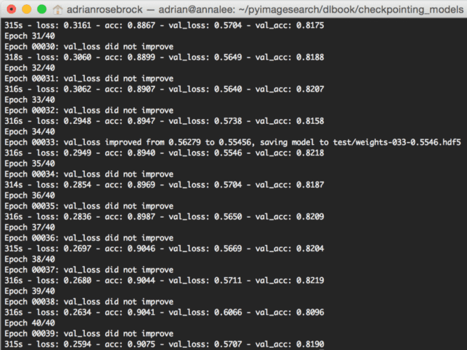
$ python cifar10_checkpoint_improvements.py --weights weights/improvements
[INFO] loading CIFAR-10 data...
[INFO] compiling model...
[INFO] training network...
Train on 50000 samples, validate on 10000 samples
Epoch 1/40
171s - loss: 1.6700 - acc: 0.4375 - val_loss: 1.2697 - val_acc: 0.5425
Epoch 2/40
Epoch 00001: val_loss improved from 1.26973 to 0.98481, saving model to test/
	weights-001-0.9848.hdf5
Epoch 40/40
Epoch 00039: val_loss did not improve
315s - loss: 0.2594 - acc: 0.9075 - val_loss: 0.5707 - val_acc: 0.8190
As we can see from my terminal output and Figure 1 , every time the validation loss decreases we save a new serialized model to disk.

Comment section
Hey, Adrian Rosebrock here, author and creator of PyImageSearch. While I love hearing from readers, a couple years ago I made the tough decision to no longer offer 1:1 help over blog post comments.
At the time I was receiving 200+ emails per day and another 100+ blog post comments. I simply did not have the time to moderate and respond to them all, and the sheer volume of requests was taking a toll on me.
Instead, my goal is to do the most good for the computer vision, deep learning, and OpenCV community at large by focusing my time on authoring high-quality blog posts, tutorials, and books/courses.
If you need help learning computer vision and deep learning, I suggest you refer to my full catalog of books and courses — they have helped tens of thousands of developers, students, and researchers just like yourself learn Computer Vision, Deep Learning, and OpenCV.
Click here to browse my full catalog.